I. Quick Review of Linear Algebra
A. A matrix is a rectangular array of numbers; a vector is a matrix with only 1 column (or only 1 row); a scalar is a matrix with 1 row and 1 column.
B. Two matrices are equal iff they have the same size and the corresponding entries in the two matrices are equal.
C. If A and B are matrices, then their sum is obtained by adding the corresponding entries in each matrix. You can only add matrices of the same size.
D. If A and B are matrices, then their product can be obtained as follows: entry (i,j) in matrix AB equals (the first element of row i in column A times the first element of column j in column B), plus (the second element of row i in column A times the second element of column j in column B)+...+(the last element of row i in column A times the last element of column j in column B). Two matrices can only be multiplied if they are conformable: to get product AB, the # of columns in A must equal the # of rows in B.  .
.
E. I is the "identity matrix" - a matrix with 1's on its diagonal and 0's everywhere else. A*I=A. A’, read "A-transpose" or "A-prime" is simply a matrix in which the 1st column of A is the first row of A’, the 2nd column of A is the second row of A’, etc.
F. A-1 is the matrix such that AA-1=I. Finding the inverse of a big matrix is extremely time consuming for a person, but computers are great at it!
G. The rank of a matrix is its number of linearly independent columns. (A set of columns is linearly independent iff ![]() has only 1 solution, with all of the k's=0).
has only 1 solution, with all of the k's=0).
H. A matrix can only be inverted if its rank is equal to its # of columns (aka if it has "full rank"). This will be very important for multiple regression, because a regression of Y on a set of variables that do not have full rank will not have a solution.
II. Multiple Regression
A. Intuitively: More than one factor often matters in the real world. And people frequently claim that some matter and others don't. Is there any way to extend the bivariate regression to shed light on this? E.g. finding the impact of IQ controlling for education, or finding the impact of spending controlling for deficits.
B. Mathematically: If you can find the "best" statistical fit between one dependent variable and one independent variable, can you find the "best" fit of one dependent variable on any number of independent variables?
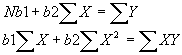
C. It is very convenient at this point to switch to matrix notation. Suppose you have N observations of all variables you are interested in. Then just write the dependent variable, Y, as a 1-column matrix (i.e., a vector) with N rows:  . And write each independent variable Xi as a vector with N rows:
  . Note further that we can think of the constant as itself one of the independent variables:
  .
.
D. Now we could write a regression equation with k variables (including the constant) as: ![]() , where b
i is the coefficient for variable i, and u is a vector of disturbance terms.
, where b
i is the coefficient for variable i, and u is a vector of disturbance terms.
E. This can be written even more compactly by combining all k columns of independent variables into one big matrix X with N rows and k columns. Similarly, combine all k coefficient scalars into a single (kx1) matrix of coefficients b
. Then we can rewrite the above equation as: ![]() !
!
F. An example: Y is a student’s grade on the final exam, and it is regressed on a constant, the # of hours the student studied, and their GPA. What do Y, X, and b look like? Are the dimensions right?
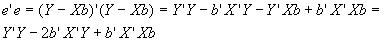 Note that Y’Xb is a scalar, so Y’Xb=b’X’Y.
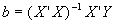 . This is an enormously powerful result.
 , then
 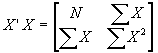 and
and 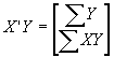 . Then
  .
. 
 will only have a solution if (X’X) is invertible. And it will only be invertible if (X’X) has full rank. But what does this mean, and is there any intuitive interpretation?
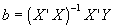 . Sub in for Y to get:
 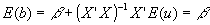 . b is an unbiased estimator for b
(given our assumptions).
. b is an unbiased estimator for b
(given our assumptions).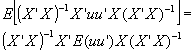 . Remembering that E(u'u)=s
2, and canceling inverses: var(b)=s
2(X'X)-1.
. Remembering that E(u'u)=s
2, and canceling inverses: var(b)=s
2(X'X)-1. , where N is the # of observations, k is the # of variables in the UN-restricted regression, k2 is the # of restrictions imposed on the 2nd regression, R2 is the R2 of the UN-restricted regression, and D
R2 is the change in the R2's.
, where N is the # of observations, k is the # of variables in the UN-restricted regression, k2 is the # of restrictions imposed on the 2nd regression, R2 is the R2 of the UN-restricted regression, and D
R2 is the change in the R2's.