Prof. Bryan Caplan
bcaplan@gmu.edu
http://www3.gmu.edu/departments/economics/bcaplan
Econ 637
Spring, 1999
Week 5: Specification Errors; Types and Transformations of Variables
- The Assumptions of OLS ("Ordinary Least Squares")
- A fussy preliminary point: the next best thing to an unbiased estimator is a consistent estimator. A consistent estimator is essentially one that becomes unbiased as N gets big. (Technically, b is consistent if plim(b)=b
).
- The econometric procedure examined in weeks 1-4 is generally known as OLS, or "ordinary least squares."
- As discussed earlier, the validity of OLS as an estimating procedure depends on certain assumptions:
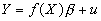
- Y=Xb
+u
- The disturbance terms ui are iid N(0,s
2)
- E(Xit,us)=0 for all i=1...k and all s,t=1...n.
- X’s are fixed (nonstochastic).
- Possible problems with u
- Problem #1: Disturbance terms are iid (0, s
2), but not normal.
- Consequences: Results from weeks 1-4 hold only asymptotically (in practice, for reasonably large samples).
- Solution(s): Get a bigger sample.
- Problem #2: Heteroscedasticity. The variance of the disturbance terms is non-constant (but still diagonal).
- Consequences: OLS remains unbiased, but becomes inefficient (higher than minimum variance).
- Solution(s): Will be examined after the midterm.
- Problem #3: Autocorrelated disturbances. E(ut,us)¹
0.
- Consequences: OLS remains unbiased, but becomes inefficient.
- Solution(s): Will be examined after the midterm.
- Possible Problems with X: The Easy Cases
- There are a number of problems with X that will yield biased estimates, but in principle as easy to remedy. Other problems require much more work to handle.
- Easy problem #1: Inclusion of irrelevant variables.
- Consequences: OLS estimates are biased. (Although as N gets large, this won't be a severe problem. Why?)
- Solution(s): Drop the irrelevant variables.
- Easy problem #2: X does not have full rank.
- Consequences: It will be impossible to invert X, so the problem will quickly be apparent.
- Solution(s): Eliminate one or more variables from X.
- Easy problem #3: "Multicollinearity." X is "close" to not having full rank.
- Consequences: This does not violate the assumptions of OLS. Your SEs will be big, but they should be!
- Solution(s): If you think you have included irrelevant variables, you can exclude them. But you should do that in any case.
- Note the parallel problem of "micronumerosity." If your number of observations N is small, you will have big SEs. And you should! You might want to get more data, but OLS is still the right procedure to use on your given tiny data set.
- Possible Problems with X: The Hard Cases
- Problem #1: "Omitted variable bias." Exclusion of relevant variables; OLS assumes that the set of k-variables includes all the variables in the true model.
- Consequences: Your estimates will be biased.
- Solution(s): Add the omitted variables. Unfortunately, you may not know what these variables are; and even if you do, there may be no available data.
- Problem #2: Correlation between X and u due to measurement error. ("Attenuation bias.")
- Consequences: Your estimates will be biased towards zero (assuming your measurement error has 0 mean).
- Solution(s): Find cleaner data; additional strategy after the midterm.
- Problem #3: Correlation between X and u because equation really ought to be part of a system of simultaneous equations. ("Simultaneity bias.")
- Consequences: Your estimates will be biased and often meaningless.
- Solutions: Will be examined after the midterm.
- Omitted Variable Bias
- Suppose the true model is
 .
.
- Partition X as [X1 X2], where X is N by k, X1 is N by k1, and X2 is N by k2.
- The first k1 coefficients may be called b1; the second k2 coefficients may be called b2.
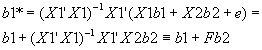
- Regressing Y on X yields: b=(X'X)-1X'Y.
- Now suppose you estimate
 .
.
- Then clearly your estimated vector for b
2 must be biased; your omission of the final variable forces it to equal zero when it is not really zero.
- What about your estimate for b
1 ? The second regression yields b1*=(X1'X1)-1X1'Y. Substituting in for Y using the equation for the true model,
 .
.
- E(b)=b
. What is E(b1*)? Taking expectations,
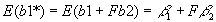 .
.
- Therefore, b1* is a biased estimator for b1, unless:
- b
2=0 (ruled out by assumption).
- F=0: the first set of variables is orthogonal to the second set. Even though both sets of variables matter, they matter in unrelated ways. (Can you think of any examples?)
- Omitted variable bias is generally a quite serious problem; it becomes even more serious when data is simply unavailable, so there is no way to figure out if you've omitted it!
- Linear Transformations and the Regression Model
- The standard regression model is written
 . Notice that this model is linear. It remains linear no matter how many independent variables you add.
- What happens to your estimate of b3 if you DOUBLE all values of X3 (where X3 is one independent variable in X)? You might do this if you changed from English to metric units of something. Or maybe you prefer to switch from writing your number in 1000's to writing it in 1,000,000's.
- Answer: The coefficient changes so that the prediction remains unchanged. If you switch from inches to feet (you divide all measurements by 12), then your coefficient increases by a factor of 12.
- What happens to your estimate of b if you DOUBLE all values of Y?
- ALL of the elements of b also double.
- What happens if you ADD the same number to all of the X3's? For example, if you decide to replace "years of college" with "years of education"?
- Answer: b3 won't change. Instead, if you add c to every value of X, the coefficient b1 on the constant falls by b3*c.
- What happens if you ADD the same number to all of the Y's?
- Answer: b2 through bk won't change, but the coefficient on the constant b1 rises by c.
- Summing up: Linear rescaling - whether by subtracting a constant from a variable, or multiplying a variable by a constant, does nothing to change the prediction. Linear changes to the regression model make no difference; they are purely a matter of convenience.
- (Verify this on 1st example).
- Doing Non-Linear Changes to a Specification
- Relations are often non-linear.
- Ex: Price increases under hyper-inflation.
- But it is possible to handle non-linear operations within the linear regression model! Just replace with
 or
or  , and estimate the new regression. As long as the coefficients are still linear, the operations that can be performed on the X's or Y's are no problem.
- Non-linear operations won't leave coefficients the same. Coefficients won't be linear functions of old coefficients, either.
- Note: you can include both a linear and a non-linear measurement of the same variable in one regression equation without violating the full rank condition.
- Ex: Common to regress earnings on Experience and Experience2 since the data show a gradual flattening of the return to education. (The coefficient on Experience is positive, the coefficient on Experience2 is negative).
- Common Non-Linear Transformations, I: Logs and Percent Changes
- Probably the most common transformation of variables is to take their natural logarithm.
- When might you want to take logs?
- If it lets you estimate the parameters of a non-linear function.
- Ex: With a standard (and non-linear!) production function Y=LaKb, taking logs leaves us with ln Y=a*ln L+ b*ln K, which looks like a standard regression problem.
- If your variable shows exponential growth over time.
- Ex: prices during a hyperinflation.
- If your variable has a big right tail.
- Ex: the distribution of income.
- Note #1: The connection between taking logs and converting variables to percent changes. Recall that the continuous growth rate of a variable is equal to [ln(Xt=T)-ln(Xt=0)]/T. Note further that for small x,
 .
.
- Thus, if you want to estimate a constant growth equation Yt=Y0(1+g)t, you can take logs of both sides of the equation, yielding ln Yt=ln Y0 + ln(1+g)t.
- Therefore, taking logs and converting variables to percentage-change form serve similar purposes. Either can be useful if it makes the results easier to interpret, or if theory suggests that percentage changes have a definite relationship:
- If a variable is constantly increasing, like many time series.
- Ex: Comparing percent change in money to the inflation rate.
- Ex: Comparing percent change in real GDP with percent change in nominal GDP.
- What is the difference between regressing Y on a constant and percent change in X, and regressing Y on a constant, ln(Xt), and ln(Xt-1)?
- Note #2: Logs are also closely related to elasticities. Recall that the elasticity of Y wrt X is dY/dX*(X/Y); it measures the percent change in Y for a percent change in X. So another reason to take logs is if you have some reason to think that an elasticity is constant.
- Ex: Suppose we begin with Y=AXb. Taking logs, we find that ln Y=ln A+b*ln X. Applying the elasticity formula, one finds that dY/dX*(X/Y)=(Y/X*b)*(X/Y)=b. So estimating the log version of the equation leaves a coefficient with a natural economic interpretation.
- Common Non-Linear Transformations, II: Lags and First Differences
- The first lag of Xt is simply Xt-1. The first lag of X in 1954 is whatever X was in 1953 (assuming you had annual data).
- You can easily include both a variable and any number of its lags as independent variables.
- Note #1: This does not violate the full rank condition.
- Note #2: N decreases by 1 for each lag you include.
- First differences: just subtract the first lag of X from X.
- Suppose that you observe me every year. Last year, you observed that I had 20 years of education and $10,000 in income. This year I have 21 years of education and $40,000 income. The first difference way of writing this is to say that YFD=+1, and IFD=$30,000.
- When do you want to do this?
- When you are worried that you have a spurious correlation.
- Ex: More educated people make more money, but does changing the education of a given person cause that person to make more money?
- If your theory predicts an effect of changes rather than levels.
- Ex: Some theories predict that the level of inflation makes no difference, but changes in the level of inflation make a difference.
- Imposing a first difference specification is equivalent to including both X and its first lag in a regression, then imposing the restriction that their coefficients be equal in magnitude but opposite in sign.
- Note the relationship between first differences and percentage changes: percentage change is identical to taking the first differences of the log of a variable. Regressing Y on a constant and percent change in X is the same as regressing Y on a constant and [ln(Xt)-ln(Xt-1)].
- Corollary: Imposing a percentage change specification is equivalent to including both ln(X) and the first lag of ln(X) in a regression, then imposing the restriction that their coefficients be equal in magnitude but opposite in sign.
- (Second example).
- Common Non-Linear Transformations, III: Squaring a Variable
- It's quite common to include both a variable and its square in a regression. When might you want to do this?
- If you variable rises at a decreasing rate (eventually the slope gets flatter).
- Ex: The effect of more years of experience: the coefficient on X is positive, the coefficient on X2 is negative. (Why doesn't this imply that earnings eventually become negative?)
- If you expect a non-linear response.
- Ex: Demand for air conditioners may rise more than linearly. 1 person buys air conditioners because average temperature rises .1 degrees, but 10,000 people buy them because it rises 10 degrees.
- Dummy Variables
- We have already briefly discussed dummy variables. A dummy variable is simply a variable that can either be 0 or 1. A dummy vector looks like: [1 0 0 1 0 0 0 1 1 1]'.
- A dummy variable is used to put "discrete" variables into a regression model. Most variables are continuous - you can earn $5 per hour, $5.07 per hour, $70.83 per hour, etc. But some variables are discrete: you either are or are not male. So if you wanted to look at the effect of "maleness," you could define a dummy variable that =1 if the person is a male, and 0 otherwise.
- Examples of Dummy Variables:
- Male = 1 if male; 0 otherwise
- White = 1 if white; 0 otherwise
- War = 1 if a country was at war in a given year; 0 otherwise
- Tall = 1 if a person is taller than 6'; 0 otherwise
- Degree =1 if a person finished their college degree; 0 otherwise ("sheepskin effect")
- Independent Dummy Variables
- You can use dummy variables as independent variables (on the right-hand side of your equation).
- If you regress one dependent variable on a constant and a dummy variable (say Male), the coefficient on the dummy variable is exactly equal to the average difference between Men and Women. If the dummy variable is $2000, it shows that men on average make $2000 more than women; if it is -$500, it shows that men on average make $500 less than women.
- If you regress one dependent variable on a dummy AND one or more other variables, then the coefficient on the dummy shows that average difference between e.g. men and women CONTROLLING for the other variables.
- You can put as many dummies as you want onto the right-hand side of your equation, but you have to be careful. You must make sure that X retains full rank; if your regression includes a constant, then your set of dummies can't sum to equal a vector of all 1's.
- E.g., you can't put both Male and Female in, because Male+Female=1. However, you could put both Male and White in, because Male+White doesn't always add up to one.
- Question: Suppose you have 50 states or 100 industries. How many "state dummies" or "industry dummies" can you include in your regression equation?
- (Third example).
- Dependent Dummy Variables
- You can also make a dummy variable the dependent variable.
- Example: regress War (=1 if the country was at war, =0 otherwise) on different economic variables to explain why countries would go to war.
- Your prediction will typically not equal either 0 or 1; rather, it will be a number in between 0 and 1. You can interpret this as the conditional probability that a country with the observed characteristics will go to war.
- Similarly, your coefficients let you estimate the marginal impact of a change in one variable for the P(Y=1).
- (This is known as the "linear probability model." It and more sophisticated techniques with the same goal will be covered later in the course).
- (Fourth example).
- Trend Variables
- Any two variables with similar trends (i.e., tendency to go up or down) will generally be highly correlated if you regress one on the other. But this is frequently bogus if given a causal interpretation: a higher price of IBM does not cause a higher price of Exxon, nor does a higher price of Exxon cause a higher price of IBM.
- Question: How can you figure out which variables with similar trends really have a significant relationship which each other?
- Answer: Add a TREND variable. A simple trend just looks like [1 2 3 4 5 ...T]'.
- If you regress e.g. the price of IBM on a trend and the price of Exxon, in all likelihood the trend will basically explain everything, and Exxon's price nothing. Exxon mattered just because it had the same general direction as IBM, not because they were really interacting.
- Similarly, you can regress e.g. real GDP on M2 and a trend. Is there really a relationship between M2 and GDP, or are they just both going up all of the time.
- (Fifth example).
- There are also more complicated trends. You can add a "quadratic trend"=[1, 4, 9, 16, 25, ...]' if a series is increasing at an increasing rate.
- Three Types of Data
- Cross sectional data: You observe each member in your sample ONCE (usually but not necessarily at the same time).
- Time series: You observe each variable once per time period for a number of periods.
- Pooled time series (="panel data"): You observe each member in your sample once per time period for a number of periods.
- Common to include "state/country/person" and "year/quarter/month" dummies. What would these look like?
- Examples of Cross Sectional Data
- Observing the heights and weights of 1000 people.
- Observing the income, education, and experience of 1000 people.
- Observing the profitability of 20 firms.
- Observing the per-capita GDP, population, and real defense spending of 80 nations.
- Examples of Time Series
- Observing U.S. inflation and unemployment from 1961-1995.
- Observing U.S. nominal GDP, real GDP, and M2 from 1960-1992.
- Observing the profitability of one firm over 20 years.
- Observing the daily closing price of gold over 30 years.
- Examples of Pooled Time Series (="panel data")
- Observing the inflation rates and rates of M2 growth of 15 countries over the 1970-1995 period.
- Observing the output and prices of 100 industries over 12 quarters.
- Observing the profitability of 20 firms over 20 years.
- Observing the annual rate of return of 300 mutual funds over the 1960-1997 period.