Bryan Caplan

bcaplan@gmu.edu

http://www3.gmu.edu/departments/economics/bcaplan

Econ 637

Spring, 1999

1. VARs, I: The Basics
1. VAR="vector autoregression." VARs are the multivariate version of univariate time series regressions.
2. General univariate autoregression simply regresses a single variable y on p lags of y:
3. General VAR works with a vector of k variables Y_t=[y1_t, y2_t, y3_t,... yk_t].
4. In a VAR, this vector Y_t is regressed on p lags of Y: .
1. Other assumptions of OLS still assumed to hold. E(e _{te s}')=W for s=t, 0 otherwise. Note: W is k by k.
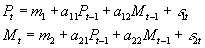
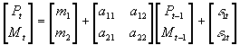
5. A VAR can be written without vector notation as a system of k equations. E.g., suppose p=1, and k=2, the two variables in question being P and M.
6. Then one could either write out:
1. A system of two equations:
2. A single vector equation with : .
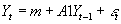3. A third way to represent the same system:
7. Just as a univariate autoregression may be stationary or nonstationary, so too may a VAR. A VAR will be stationary so long as the modulus of each of the eigenvalues of A is less than 1. (You may skip discussion of alternative cases in text).
1. Brief refresher: eigenvalues are the values of lambda that solve the equation:
.
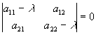
8. Punchline: So long as VAR is stationary, you can estimate the coefficients and SEs by separately applying OLS to each equation in the system! (This is one of the special cases where SUR and OLS yield identical results).
2. VARs, II: Granger Causality and Impulse Response Functions
1. The way VARs are set up makes it natural to test for so-called "Granger causality," a misnomer since it has nothing to do with causality. Rather: y2 Granger causes y1 if a regression of y1 on lagged y2 yields a coefficient significantly different from zero.
1. A slightly more involved test of pseudo-causality: see if lagged y2 predicts y1, but lagged y1 does not predict y2.
2. One interesting thing about VARs (and system of equations more generally) is that even though the system is linear, a disturbance can affect the system in non-linear ways. When you calculate the response of the system to a shock, you are calculating the impulse response function.
3. One simple example (from Johnston/DiNardo). Suppose you have a 2-variable, 1-lag VAR: 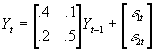. Ceteris paribus, what happens to the system if at t=0, e _1t=1?
4. Implement the ceteris paribus assumption by setting all disturbances except e _1t equal to 0, along with all lags of Y_t before t=0.
5. Then in t=0, .
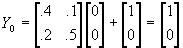6. But then at t=1, 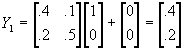; at t=2, 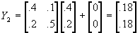; at t=3, 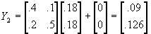, etc. Thus a single shock to one linear equation set of a "chain reaction" throughout the system.
7. The shock could also have been from an exogenous variable added to the VAR system rather than from the realization of the error term.
8. General procedure for calculating ir's:
1. Initially set everything equal to 0 except your shock. This includes your lagged Y's for p periods into the past.
2. Calculate Y₀ using the equations of your linear system.
3. Calculate subsequent values of Y by plugging past values of Y into your linear system. When programming, an iterative procedure is natural: calculate Y₀, set Y_-1, Y_-2, Y_-p to all zeros. Then set up a loop to have the computer calculate Y₁ using Y₀ through Y_-p+1, then calculate Y₂ using Y₁ through Y_-p+2, etc.
3. Standard Error Bands
1. Once you calculate and graph your impulse-response function, you might like to get some notion of the precision with which your i-r has been estimated.
2. So, people frequently add "SE bands" to show upper and lower bounds for the probable response of the system to a given shock.
3. SE bands are derived from the original coefficients and their SEs. Essentially, you are imagining how the system would behave if it turned out that your estimates were different in plausible ways.
4. Several different ways to calculate SE bands. Easiest if your software isn't smart enough to do the work for you:
1. Use approximation for the variance of a function of a vector of coefficients b: f'(b)'*V(b)*f'(b). V is the variance-covariance matrix for b, and f'(b) is the matrix of numerical derivatives for a given ir.
5. My version is Eviews is smart enough to calculate SE bands for VARs but not for systems of equations in general.
4. VARs and Causation
1. How do VARs solve the simultaneity problem endemic to the estimation of systems of equations? Some misunderstanding to the contrary, VARs alone do nothing to solve this problem.
2. VARs usefully summarize data, just as regressing Q on P may usefully summarize data. Both may be useful for predictions, but they tell us nothing about causality.
3. One popular way to try to convert VARs into tools of causal inference has been to use "orthogonalized innovations." (See text for more detailed treatment).
4. With the orthogonalized innovations, a shock to the 1^st error implies a shock to the 2^nd; but a shock to the 2^nd does not imply a shock to the first. Many have found this econometric procedure to be causally instructive.
1. If you think that money contemporaneously causes prices to increase, but don't think that prices contemporaneously causes money to increase, then put M first and P second. Then a shock to P won't contemporaneously change M, but a shock to M will contemporaneously change P.
5. Ex: Bernanke-Blinder (1992) - solving simultaneity of non-policy and policy variables by assuming either no contemporaneous impact of non-policy on policy, or no contemporaneous impact of policy on non-policy.
6. But: this procedure generates great controversy, because you typically have to assume what you want to prove - i.e., the direction of causation!
7. When VARs have a causal interpretation, they are often called "structural" VARs, or SVARs. Using orthogonalized innovations is perhaps the most popular strategy for getting SVARs.
5. Systems of Simultaneous Equations and Causation
1. Regular VARs have no causal interpretation; SVARs do.
2. Instead of assuming orthogonalized innovations to give your VAR a causal interpretation, you can simply apply standard principles of identification, learned in weeks 8-9.
3. Once you estimate all of the equations in your system, you can then calculate the impulse response function, SE bands, and give your VAR a causal interpretation.
4. The same applies if you have a system of time series equations that don't look like VARs. Use standard principles of identification to give your results a causal interpretation. Then, calculate the ir function and SE bands.