Prof.
Bryan Caplan
bcaplan@gmu.edu
http://www.bcaplan.com
Econ
854
Week 5: Voter Motivation, II:
Ideological Voting
I.
Factor Analysis
A.
One statistical technique social scientists outside of economics use a
great deal is factor analysis.
B.
The main idea of factor analysis: reducing a lot of variables to a
smaller number of "summary" variables, aka "factors" or
"dimensions."
C.
The classic example: intelligence testing. A test has 100 items. Is it possible to extract a smaller
number of summary variables?
D.
Yes. In fact, factor
analysis on variables related to cognitive ability normally finds ONE
over-riding factor (called g for "general intelligence"). Cognitive ability is essentially
"one-dimensional."
E.
Performance on individual test items can be seen as a function of g
plus noise. The greater the
predictive power of g, the higher we say the item's g-loading is.
1.
Ex: Analogies have a higher g-loading than pure memory tasks.
F.
Factor analysis in no way guarantees the existence of a single
over-riding factor. For example, on
personality tests, factor analysis normally extracts FIVE unrelated
factors.
G.
Factors do not label themselves.
Ordinary language terms are convenient, though occasionally misleading.
1.
Ex: OCEAN
H.
On purely random data, no factors would emerge.
II.
The Dimensionality of
A.
There are many different ways to analyze political beliefs.
1.
Libertarian-statist spectrum
2.
Christian-secular spectrum
B.
What can factor analysis tell us about the dimensionality of
C.
Strong result: As with intelligence, empirical tests typically find
that political opinion is roughly one dimensional.
D.
What is the dimension?
Empirically,
B.
On a deep level, this spectrum may not make a great deal of sense. Libertarians, for example, often argue
that there are really two dimensions - personal freedom and economic freedom:
1.
Libertarians - pro-personal, pro-economic
2.
Populists - anti-personal, anti-economic
3.
Liberals - pro-personal, anti-economic
4.
Conservatives - anti-personal, pro-economic
E.
But empirically, most people line up on the diagonal, and the other two
boxes are sparsely inhabited.
F.
G.
A second dimension (related to race) occasionally pops up, but is no
longer important. P&R's story:
During the 50's, otherwise liberal Southern Democrats often opposed civil
rights measures, and otherwise conservative Republicans often favored them. Once the Southern Democrats left the
party, and debate shifted from "equality of opportunity" to
"equality of result," position on further civil rights measures began
to correlate well with the rest of the liberal-conservative dimension.
H.
Similarly, Levitt and earlier researchers have found that
one-dimensional ideological measures of l-c like
I.
Less work has been done on the dimensionality of individual citizens'
opinions, but once again, a strong liberal-conservative dimension pops out of
the data.
J.
Remarkably, voting in the U.N. is also one-dimensional, in spite of the
extreme heterogeneity of the participants.
The dimension is something like "attitudes towards the
U.S./Israel."
III.
Ideological Voting
A.
As mentioned earlier, the main problem with the simple sociotropic
voting model is that it has trouble explaining disagreement.
B.
The empirical evidence on ideology suggests a more sophisticated
interpretation of sociotropic voting.
C.
Motivation is indeed sociotropic: People support the policies they
think are in the public interest.
D.
But: There are large ideological disagreements about the public
interest. Ideology determines
beliefs about what policies "work" and what counts as
"working."
E.
Ex: Affirmative action.
Conservatives and liberals argue about whether it works (are blacks
better-off because of it?), but also disagree about what it means to
"work" (a "level playing field" versus a "fair
outcome"?).
F.
Important theoretical point: If ideology is one-dimensional, and people
largely vote ideologically, then the simple MVT's seemingly strong assumptions
are satisfied. Perhaps the
issue-space only looks multi-dimensional.
V.
Ideology and Reduction
A.
Main objection to ideological voting model: Can't ideology be reduced
to personal interests?
B.
Ex: Isn't conservatism just the "ideology of the rich," and
liberalism the "ideology of the poor"?
C.
No. The correlation between
income and professed ideology is very low.
In the GSS, for example, the correlation between real income and
POLVIEWS (a 1-7 measure of left-right ideology) is .06.
D.
So what does determine ideology?
Is it education?
E.
Once again, no. Education
and ideology are close to unrelated (r=-.03) when you look at a random sample of
Americans from the GSS (as opposed to, say, a 50/50 sample of random Americans
and university faculty!).
F.
In a multiple regression framework, there is a tendency for income to
make people more conservative and education to make people more liberal. [Table 2]
G.
Both are clearly statistically significant, but the actual effect is
small. On a 6-point scale:
1.
Raising log of real income by 1 – a huge change - makes people
.096 units more conservative.
2.
Going from a high school degree to a BA makes people .084 units more
liberal.
H.
What then is ideology? As
far as anyone can show, ideology is an independent causal force. Ideology explains a great deal about
people's beliefs, but no standard social science variable does much to explain
ideology.
I.
Maybe someone will one day show that ideology reduces to something
else, but given the failure of all the obvious candidates, I doubt it. (But stay tuned for the genetics of politics
next week!)
VI.
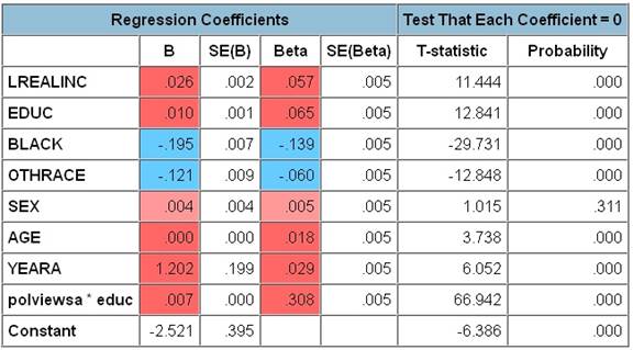
Case Study: The Determinants of Party Identification, II
A.
Question: Returning to last
week's linear probability model of party identification, what happens in the
GSS if you also control for stated ideology? N≈41,000,
so focus on magnitudes, not t-stats.
B.
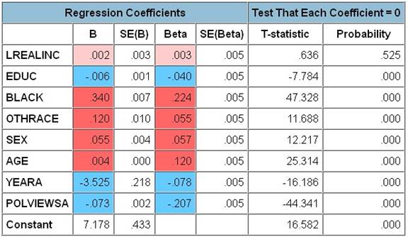
[Tables 3a&3b]
C.
Answer: Ideology matters
even more than race. Moreover, the
slight change in the other coefficients shows that ideology is far from a
"mere proxy for self-interest."
D.
Consider two examples for 2010.
1.
Ex. #1: Black female with
$1M annual income in 1986 dollars, 30 years old, college graduate.
2.
Ex. #2: White male with
$10k annual income, 30 years old, high school education, conservative ideology.
E.
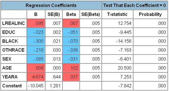
Ex. #1: [Since we don't
know ideology, use Tables 1a and 1b]
Estimated probability of being a Democrat: 56.4%; estimated probability
of being a Republican: 26.6%.
F.
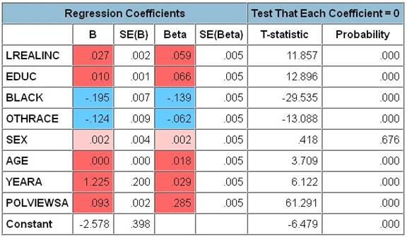
Ex. #2: [Using Tables 3a
and 3b] Estimated probability of
being a Democrat: 6.8%; estimated probability of being a Republican: 59.1%. (Age coefficient to one more decimal
place=.0005).
VII.
Income, Education, Ideology, and Opinion
A.
For specific opinions (as opposed to party identification), income
empirically often seems to make a large difference.
1.
Ex: High income people seem much more in favor of immigration than low
income people.
B.
But
the effect of income almost always disappears once you control for education. Ph.D.s who drive cabs think like other
Ph.D.s, not other cab drivers.
C.
How does education affect opinion? More educated people tend to be
both more tolerant and more appreciative of free markets.
D.
Even though voting is one-dimensional, opinion looks
two-dimensional.
E.
Moreover, the two dimensions more or less fit the two-dimensional
personal freedom/economic freedom diagram.
Education shifts the diagonal up and to the right.
F.
This fact suggests that politicians might really compete over two
dimensions rather than one, again raising doubts about the median voter model.
G.
In practice, however, the liberal-conservative dimension appears to be
far more electorally salient.
Education affects issue beliefs, but appears to be independent of party
identification.
H.
Why? How come liberals
ally, but not high school drop-outs?
VIII.
Case Study: Economic Beliefs
A.
Now let us go through two illustrations from the SAEE: tendency to
blame economic difficulties on:
1.
Immigration
2.
"Excessive profits"
B.
If we do not control for education, income appears to have a large effect
on these beliefs. [Table 4a, 4b]
C.
Controlling for education, though, makes the apparent effect of income
almost disappear. [Table 5a, 5b]
D.
Immigration.
1.
Opposition shrinks as education rises.
2.
Opposition grows as conservatism rises.
E.
"Excessive profits."
1.
Assigning blame falls as education rises.
2.
Assigning blame falls as conservatism rises.
IX.
The Ideology*Education Interaction
A.
Ideology and education interact in an interesting way. Despite their slight correlation,
ideology*education has more predictive power than ideology alone.
B.
Simple explanation: The higher your education level, the more likely
you are to know what your ideology says about a given topic. For someone with a grade-school
education, "liberal" is just a word; for a Ph.D., it is an integrated
worldview.
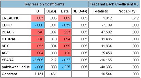
C.
This works for party identification: The tstat on ideology*education is
higher than the tstat on ideology alone, rising from 44 and 61 to 48 and 67. [Tables
3a&3b vs. Tables 6a&6b]
D.
It also works on individual issues. For immigration, the tstat rises from
3.9 to 4.3 [Table 4a versus 7a]; for excessive profits, from 4.6 to 4.9 [Table
4b versus 7b].
E.
Returning to the two-dimensional diagram, education
"stretches" the liberal-conservative spectrum.
Table
2: The Determinants of Ideology (POLVIEWS rescaled to go from -3 to +3)
Table
3a: Conditional Probability of Being a Democrat, with Ideology
Table
3b: Conditional Probability of Being a Republican, with Ideology
Table
4a: Effect of Income on Beliefs About Immigration, No Education Control
|
Dependent Variable: IMMIG |
|
||||
|
Method: Least Squares |
|
||||
|
Date: 10/23/01 Time: 13:02 |
|
||||
|
Sample(adjusted): 1 1510 IF ECON<1 |
|
||||
|
Included observations: 1362 after
adjusting endpoints |
|
||||
|
Variable |
Coefficient |
Std. Error |
t-Statistic |
Prob. |
|
|
C |
1.581155 |
0.176059 |
8.980843 |
0.0000 |
|
|
BLACK |
-0.141790 |
0.076408 |
-1.855686 |
0.0637 |
|
|
ASIAN |
-0.002224 |
0.092337 |
-0.024084 |
0.9808 |
|
|
OTHRACE |
-0.004465 |
0.090074 |
-0.049576 |
0.9605 |
|
|
AGE |
-0.009174 |
0.007457 |
-1.230223 |
0.2188 |
|
|
AGE^2 |
0.000139 |
7.59E-05 |
1.832582 |
0.0671 |
|
|
MALE |
-0.130501 |
0.042039 |
-3.104298 |
0.0019 |
|
|
IDEOLOGY*(1-OTHIDEOL) |
0.106427 |
0.023119 |
4.603419 |
0.0000 |
|
|
OTHIDEOL |
0.242322 |
0.150883 |
1.606028 |
0.1085 |
|
|
JOBWORRY |
0.049389 |
0.019877 |
2.484734 |
0.0131 |
|
|
YOURFAM5 |
-0.018488 |
0.033123 |
-0.558180 |
0.5768 |
|
|
YOURNEXT5 |
-0.037205 |
0.033983 |
-1.094799 |
0.2738 |
|
|
INCOME |
-0.041745 |
0.010383 |
-4.020541 |
0.0001 |
|
|
R-squared |
0.069468 |
Mean dependent var |
1.218796 |
|
|
|
Adjusted R-squared |
0.061191 |
S.D. dependent var |
0.779419 |
|
|
|
S.E. of regression |
0.755196 |
Akaike info criterion |
2.285819 |
|
|
|
Sum squared resid |
769.3625 |
Schwarz criterion |
2.335612 |
||
|
Log likelihood |
-1543.643 |
F-statistic |
8.392399 |
||
|
Durbin-Watson stat |
2.049180 |
Prob(F-statistic) |
0.000000 |
||
Table
4b: Effect of Income on Beliefs About “Excessive Profits,” No
Education Control
|
Dependent Variable: PROFHIGH |
||||
|
Method: Least Squares |
||||
|
Date: 10/23/01 Time: 13:02 |
||||
|
Sample(adjusted): 1 1510 IF ECON<1 |
||||
|
Included observations: 1355 after
adjusting endpoints |
||||
|
Variable |
Coefficient |
Std. Error |
t-Statistic |
Prob. |
|
C |
1.346526 |
0.164472 |
8.186947 |
0.0000 |
|
BLACK |
0.078105 |
0.071559 |
1.091486 |
0.2753 |
|
ASIAN |
-0.011367 |
0.087285 |
-0.130229 |
0.8964 |
|
OTHRACE |
0.160538 |
0.085611 |
1.875199 |
0.0610 |
|
AGE |
0.010419 |
0.006962 |
1.496472 |
0.1348 |
|
AGE^2 |
-7.23E-05 |
7.09E-05 |
-1.020087 |
0.3079 |
|
MALE |
-0.202624 |
0.039320 |
-5.153159 |
0.0000 |
|
IDEOLOGY*(1-OTHIDEOL) |
-0.090241 |
0.021657 |
-4.166787 |
0.0000 |
|
OTHIDEOL |
0.180299 |
0.140710 |
1.281355 |
0.2003 |
|
JOBWORRY |
0.037830 |
0.018623 |
2.031381 |
0.0424 |
|
YOURFAM5 |
-0.056647 |
0.030934 |
-1.831217 |
0.0673 |
|
YOURNEXT5 |
-0.104313 |
0.031768 |
-3.283568 |
0.0011 |
|
INCOME |
-0.036220 |
0.009713 |
-3.729038 |
0.0002 |
|
R-squared |
0.108802 |
Mean dependent var |
1.272325 |
|
|
Adjusted R-squared |
0.100833 |
S.D. dependent var |
0.742522 |
|
|
S.E. of regression |
0.704092 |
Akaike info criterion |
2.145732 |
|
|
Sum squared resid |
665.2902 |
Schwarz criterion |
2.195732 |
|
|
Log likelihood |
-1440.733 |
F-statistic |
13.65318 |
|
|
Durbin-Watson stat |
2.008430 |
Prob(F-statistic) |
0.000000 |
|
Table
5a: Effect of Income on Beliefs About Immigration, Education Control
|
Dependent Variable: IMMIG |
||||
|
Method: Least Squares |
||||
|
Date: 10/23/01 Time: 12:49 |
||||
|
Sample(adjusted): 1 1510 IF ECON<1 |
||||
|
Included observations: 1362 after
adjusting endpoints |
||||
|
Variable |
Coefficient |
Std. Error |
t-Statistic |
Prob. |
|
C |
1.883690 |
0.174664 |
10.78466 |
0.0000 |
|
BLACK |
-0.174951 |
0.074420 |
-2.350864 |
0.0189 |
|
ASIAN |
0.035971 |
0.089924 |
0.400013 |
0.6892 |
|
OTHRACE |
-0.032613 |
0.087676 |
-0.371975 |
0.7100 |
|
AGE |
-0.004571 |
0.007273 |
-0.628464 |
0.5298 |
|
AGE^2 |
8.37E-05 |
7.41E-05 |
1.129602 |
0.2588 |
|
MALE |
-0.115403 |
0.040928 |
-2.819625 |
0.0049 |
|
IDEOLOGY*(1-OTHIDEOL) |
0.088741 |
0.022578 |
3.930411 |
0.0001 |
|
OTHIDEOL |
0.253523 |
0.146774 |
1.727304 |
0.0843 |
|
JOBWORRY |
0.036076 |
0.019394 |
1.860182 |
0.0631 |
|
YOURFAM5 |
0.004961 |
0.032329 |
0.153453 |
0.8781 |
|
YOURNEXT5 |
-0.025312 |
0.033084 |
-0.765072 |
0.4444 |
|
INCOME |
-0.011501 |
0.010667 |
-1.078253 |
0.2811 |
|
EDUCATION |
-0.121877 |
0.013828 |
-8.814086 |
0.0000 |
|
R-squared |
0.120175 |
Mean dependent var |
1.218796 |
|
|
Adjusted R-squared |
0.111690 |
S.D. dependent var |
0.779419 |
|
|
S.E. of regression |
0.734604 |
Akaike info criterion |
2.231255 |
|
|
Sum squared resid |
727.4387 |
Schwarz criterion |
2.284878 |
|
|
Log likelihood |
-1505.485 |
F-statistic |
14.16323 |
|
|
Durbin-Watson stat |
2.020208 |
Prob(F-statistic) |
0.000000 |
|
Table
5b: Effect of Income on Beliefs About “Excessive Profits,”
Education Control
|
Dependent Variable: PROFHIGH |
||||
|
Method: Least Squares |
||||
|
Date: 10/23/01 Time: 12:49 |
||||
|
Sample(adjusted): 1 1510 IF ECON<1 |
||||
|
Included observations: 1355 after
adjusting endpoints |
||||
|
Variable |
Coefficient |
Std. Error |
t-Statistic |
Prob. |
|
C |
1.509230 |
0.166386 |
9.070651 |
0.0000 |
|
BLACK |
0.060476 |
0.071038 |
0.851317 |
0.3947 |
|
ASIAN |
0.008011 |
0.086629 |
0.092480 |
0.9263 |
|
OTHRACE |
0.144138 |
0.084945 |
1.696828 |
0.0900 |
|
AGE |
0.012815 |
0.006920 |
1.851821 |
0.0643 |
|
AGE^2 |
-0.000101 |
7.05E-05 |
-1.432204 |
0.1523 |
|
MALE |
-0.194440 |
0.039020 |
-4.983073 |
0.0000 |
|
IDEOLOGY*(1-OTHIDEOL) |
-0.099322 |
0.021551 |
-4.608611 |
0.0000 |
|
OTHIDEOL |
0.185962 |
0.139513 |
1.332934 |
0.1828 |
|
JOBWORRY |
0.030960 |
0.018516 |
1.672024 |
0.0948 |
|
YOURFAM5 |
-0.044179 |
0.030774 |
-1.435562 |
0.1514 |
|
YOURNEXT5 |
-0.097896 |
0.031524 |
-3.105476 |
0.0019 |
|
INCOME |
-0.020394 |
0.010153 |
-2.008678 |
0.0448 |
|
EDUCATION |
-0.064849 |
0.013178 |
-4.920943 |
0.0000 |
|
R-squared |
0.124610 |
Mean dependent var |
1.272325 |
|
|
Adjusted R-squared |
0.116123 |
S.D. dependent var |
0.742522 |
|
|
S.E. of regression |
0.698080 |
Akaike info criterion |
2.129311 |
|
|
Sum squared resid |
653.4895 |
Schwarz criterion |
2.183157 |
|
|
Log likelihood |
-1428.608 |
F-statistic |
14.68370 |
|
|
Durbin-Watson stat |
2.000165 |
Prob(F-statistic) |
0.000000 |
|
Table
6a: Conditional Probability of Being a Democrat, with Ideology*Educ
Table
6b: Conditional Probability of Being a Republican, with Ideology*Educ
Table
7a: Effect of Income on Beliefs About Immigration, Ideology*Educ Interaction
|
Dependent Variable: IMMIG |
||||
|
Method: Least Squares |
||||
|
Date: 10/23/01 Time: 12:54 |
||||
|
Sample(adjusted): 1 1510 IF ECON<1 |
||||
|
Included observations: 1362 after
adjusting endpoints |
||||
|
Variable |
Coefficient |
Std. Error |
t-Statistic |
Prob. |
|
C |
1.901975 |
0.174285 |
10.91305 |
0.0000 |
|
BLACK |
-0.167020 |
0.074339 |
-2.246730 |
0.0248 |
|
ASIAN |
0.038885 |
0.089935 |
0.432370 |
0.6655 |
|
OTHRACE |
-0.032774 |
0.087630 |
-0.374001 |
0.7085 |
|
AGE |
-0.004735 |
0.007263 |
-0.651871 |
0.5146 |
|
AGE^2 |
8.50E-05 |
7.40E-05 |
1.148399 |
0.2510 |
|
MALE |
-0.116930 |
0.040887 |
-2.859876 |
0.0043 |
|
IDEOLOGY*(1-OTHIDEOL)*EDUCATION |
0.020108 |
0.004718 |
4.261634 |
0.0000 |
|
OTHIDEOL*EDUCATION |
0.062666 |
0.032606 |
1.921896 |
0.0548 |
|
JOBWORRY |
0.036512 |
0.019397 |
1.882333 |
0.0600 |
|
YOURFAM5 |
0.005987 |
0.032285 |
0.185437 |
0.8529 |
|
YOURNEXT5 |
-0.025103 |
0.033047 |
-0.759605 |
0.4476 |
|
INCOME |
-0.011887 |
0.010661 |
-1.114952 |
0.2651 |
|
EDUCATION |
-0.124634 |
0.013817 |
-9.020040 |
0.0000 |
|
R-squared |
0.122481 |
Mean dependent var |
1.218796 |
|
|
Adjusted R-squared |
0.114018 |
S.D. dependent var |
0.779419 |
|
|
S.E. of regression |
0.733641 |
Akaike info criterion |
2.228631 |
|
|
Sum squared resid |
725.5321 |
Schwarz criterion |
2.282253 |
|
|
Log likelihood |
-1503.698 |
F-statistic |
14.47294 |
|
|
Durbin-Watson stat |
2.021390 |
Prob(F-statistic) |
0.000000 |
|
Table
7b: Effect of Income on Beliefs About “Excessive Profits,”
Ideology*Educ Interaction
|
Dependent Variable: PROFHIGH |
||||
|
Method: Least Squares |
||||
|
Date: 10/23/01 Time: 12:54 |
||||
|
Sample(adjusted): 1 1510 IF ECON<1 |
||||
|
Included observations: 1355 after
adjusting endpoints |
||||
|
Variable |
Coefficient |
Std. Error |
t-Statistic |
Prob. |
|
C |
1.504577 |
0.166017 |
9.062768 |
0.0000 |
|
BLACK |
0.048497 |
0.070958 |
0.683463 |
0.4944 |
|
ASIAN |
-0.004565 |
0.086640 |
-0.052685 |
0.9580 |
|
OTHRACE |
0.135789 |
0.084901 |
1.599375 |
0.1100 |
|
AGE |
0.013030 |
0.006910 |
1.885486 |
0.0596 |
|
AGE^2 |
-0.000104 |
7.04E-05 |
-1.471935 |
0.1413 |
|
MALE |
-0.192414 |
0.038981 |
-4.936041 |
0.0000 |
|
IDEOLOGY*(1-OTHIDEOL)*EDUCATION |
-0.022115 |
0.004490 |
-4.924966 |
0.0000 |
|
OTHIDEOL*EDUCATION |
0.049965 |
0.030994 |
1.612075 |
0.1072 |
|
JOBWORRY |
0.028983 |
0.018517 |
1.565193 |
0.1178 |
|
YOURFAM5 |
-0.046264 |
0.030730 |
-1.505501 |
0.1324 |
|
YOURNEXT5 |
-0.096444 |
0.031489 |
-3.062790 |
0.0022 |
|
INCOME |
-0.019645 |
0.010146 |
-1.936233 |
0.0530 |
|
EDUCATION |
-0.065029 |
0.013171 |
-4.937448 |
0.0000 |
|
R-squared |
0.126969 |
Mean dependent var |
1.272325 |
|
|
Adjusted R-squared |
0.118506 |
S.D. dependent var |
0.742522 |
|
|
S.E. of regression |
0.697138 |
Akaike info criterion |
2.126612 |
|
|
Sum squared resid |
651.7280 |
Schwarz criterion |
2.180458 |
|
|
Log likelihood |
-1426.780 |
F-statistic |
15.00220 |
|
|
Durbin-Watson stat |
2.001392 |
Prob(F-statistic) |
0.000000 |
|