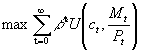
 ; an infinitely-lived agent derives utility from consumption and real balances.
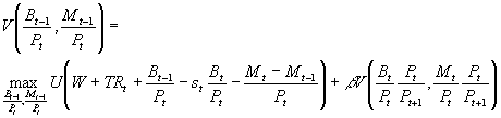
Prof. Bryan Caplan
bcaplan@gmu.eduhttp://www3.gmu.edu/departments/economics/bcaplan
Econ 918
Spring, 1998
Week 1: Theories of Money Demand
; an infinitely-lived agent derives utility from consumption and real balances. .
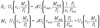
. . It then follows that real money demand falls when the rate of money creation rises, AND when the discount factor falls (i.e., people get more impatient).