Prof. Bryan Caplan

bcaplan@gmu.edu

http://www3.gmu.edu/departments/economics/bcaplan

Econ 816

Spring, 2000

 

HW#4 Answers

 

Part 1: Mathematical Problems

1.  Romer, problem 9.8.

 

a.  Since this is an RE model without exogenous uncertainty, the fact that expected inflation p^e=b/a implies that actual inflation p=b/a.  Therefore,  .

 

b.  The AS function in the intial period will be:

 

 

 

The 1-period OF is therefore:

 

 

Differentiating:

 

, so

 

Plugging into the lifetime OF yields:

 

 

Whereas if the policymaker did not defect, lifetime OF would be:

 

 

c.  Find when :

 

 

Cancelling and simplifying:

 

 

 

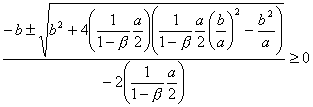
This leaves us with a quadratic equation in .  Solve using the quadratic formula, it can be seen that the above inequality holds if:

 

 

Simplifying:

 

 

 

The two critical values are thus:  and .

 

Cooperation will then be possible so long as:

 

.

 

If , it cannot be larger than b/a, so equilibrium will exist so long as:

 

, implying that .

 

 

2.  Romer, problem 9.9.

 

In all three problems, the cooperation utility remains:

 

 

a.  Defection will only pay if one can defect one period, take the punishment for one period, and be better off than if one had cooperated.  So compare:

 

 to:

 

Simplifying:

 

 

 

Again solving the quadratic equation for the critical values (and simplifying!):

 

, so the critical values are  and .

 

Cooperation will then be possible so long as:

 

.

 

b. This implies a two-period cost of defection.  For convenience, define .  Then compare:

 

 to:

 

 

So in equilibrium:

 

Simplifying:

 

 

 

Applying the quadratic formula yields the following mess:

 

 

Which shows that with extreme punishments, you can get cooperation in more general circumstances than you can otherwise.

 

c.  This is always an equilibrium; in each period, the policy-maker is optimizing relative to the public's actions, and vice versa.

 

3.  Romer, problem 9.16.

 

ln(M_t/P_t)=a-bi+ln Y_t, so:

 

M_t/P_t=e^a-biY_t

 

i=r+p^e

 

The percent change in the money supply plus the inflation rate must equal the real rate of growth, so:

 

p=g_M-g_Y

 

i=r+g_M-g_Y

 

Plugging into the equation for real balances:

 

M_t/P_t=exp(a)exp(-b[r+g_M-g_Y])Yt

 

Seigniorage equals the change in real balances:

 

 

Plugging in:

 

S=g_M*exp(a)exp(-b[r+g_M-g_Y])Yt

 

Then just maximize S wrt g_M, getting:

 

[exp(a)exp(-b[r+g_M-g_Y])Yt]-bg_M[exp(a)exp(-b[r+g_M-g_Y])Yt]=0

 

Thus:

 

[exp(a)exp(-b[r+g_M-g_Y])Yt][1-bg_M]=0

 

The first term in brackets is always positive, so the only solution is given by:

 

[1-bg_M]=0

 

Implying g_M*=1/b

 

4.  Romer, problem 9.17.

 

a. As in the last problem, .

Define  and .  Then

 

Next, note that inflation is just the difference between nominal money growth and real money growth:

 

Let G be the amount of seigniorage the government spends:

 

, so

 

The money demand equation can be used to compute :

 

Plugging into the equation for inflation:

 

 

Now plug the above into the equation for the change in expected inflation:

 

, so:

 

Re-arranging terms:

 

 

 

b.  In this case, you essentially get a hyperinflation - every period to have to make inflation higher to get more than S* in revenue.

 

c.  Now in the steady state, expected inflation equals actual inflation equals the rate of money growth.